Lagrange interpolation polynomial. Interpolation of a function by Lagrange polynomials Purpose of laboratory work
Let on the segment function y=f(x) is given in a table, i.e. (x i , y i), (i=0,1,..,n), Where y i =f(x i). This given function is called " mesh».
Formulation of the problem: find algebraic polynomial (polynomial):
degree no higher n such that
L n (x i)=y i , at i= 0,1,..,n,(5.6)
those. having at given nodes xi, (i=0,1,..,n) same values as the grid function at=f(x).
The polynomial itself Ln(x) called interpolation polynomial, and the task is polynomial interpolation .
Find the polynomial L n (x)- this means find its coefficients a 0 , a 1 ,…,a n. For this there is n+ 1 condition (5.6), which are written as a system of linear algebraic equations for unknowns a i,(i=0, 1,…,n):

Where x i and y i ( i=0,1,…,n) – table values of argument and function.
From an algebra course we know that the determinant of this system, called the Vandermonde determinant:

non-zero and, therefore, system (5.7) has only decision.
Having determined the coefficients a 0 , a 1 ,…,a n, solving system (5.7), we obtain the so-called Lagrange interpolation polynomial for function f(x):
![]() (5.8)
(5.8)
which can be written as:
It is proved that given n+1 function values can be plotted Lagrange's only interpolation polynomial(5.8).
In practice, Lagrange interpolation polynomials of the first ( n= 1) and second ( n= 2) degrees.
At n= 1 information about the interpolated function y=f(x) is specified at two points: (x 0 , y 0 ) and (x 1 , y 1 ), and the Lagrange polynomial has the form
For n= 2 Lagrange polynomial is constructed using the three-point table
Solution: We substitute the initial data into formula (5.8). The degree of the resulting Lagrange polynomial is not higher than third, since the function is specified by four values:
![]()
Using the Lagrange interpolation polynomial, you can find the value of the function at any intermediate point, for example at X=4:
![]() = 43
= 43
Lagrange interpolation polynomials used in finite element method, widely used in solving construction problems.
Other interpolation formulas are also known, for example, Newton's interpolation formula, used for interpolation in the case of equidistant nodes or interpolation polynomial Ermita.
Spline interpolation. When using a large number of interpolation nodes, a special technique is used - piecewise polynomial interpolation, when the function is interpolated by a polynomial of degree T between any adjacent grid nodes.
Root mean square approximation of functions
Formulation of the problem
RMS approximation functions is another approach to obtaining analytical expressions for approximating functions. A feature of such problems is the fact that the initial data for constructing certain patterns are obviously approximate character.
This data is obtained as a result of some experiment or as a result of some computational process. Accordingly, these data contain experimental errors (errors in measuring equipment and conditions, random errors, etc.) or rounding errors.
Let's say we are investigating some phenomenon or process. In general terms, the object of research can be represented by a cybernetic system (“black box”) shown in the figure.
Variable X is an independent, controlled variable (input parameter).
Variable Y– this is the reaction (response) of the object of study to the influence of the input parameter. This is the dependent variable.
Let us assume that when processing the results of this experiment, a certain functional dependence is discovered y=f(x) between independent variable X and dependent variable u. This dependence is presented in the form of a table. 5.1 meanings x i , y i (i=1,2,…,n) obtained during the experiment.
Table 5.1
| x i | x 1 | x 2 | … | x n |
| y i | y 1 | y 2 | … | y n |
If the analytical expression of the function y=f(x) unknown or very difficult, then the task arises of finding the function y= j (X), whose values at x=x i, maybe it was a little different based on experimental data y i , (i=1,..,n). Thus, the dependence under study is approximated by the function y= j (X) on the segment [ x 1 ,xn]:
f(x)@ j (X). (5.9)
Approximation function y= j (X) called empirical formula (EF) or regression equation (RE).
Empirical formulas do not pretend to be laws of nature, but are only hypotheses that more or less adequately describe experimental data. However, their significance is very great. There are cases in the history of science when the resulting successful empirical formula led to great scientific discoveries.
The empirical formula is adequate, if it can be used to describe the object under study with sufficient accuracy for practice.
What is this dependence for?
If approximation (5.9) is found, then it is possible:
Make a prediction about the behavior of the object under study outside the segment ( extrapolation );
Choose optimal direction of development of the process under study.
The regression equation can have different forms and different levels of complexity depending on the characteristics of the object under study and the required accuracy of representation.
Geometrically The task of constructing a regression equation is to draw a curve L: y= j (X) « perhaps closer» adjacent to the system of experimental points M i (x i , y i), i= 1,2,..,n, given by the table. 5.1 (Fig. 5.2).
Construction of a regression equation (empirical function) consists of 2 stages:
1. general view selection regression equations,
2. determining its parameters.
Successful choice The regression equation largely depends on the experience of the experimenter studying any process or phenomenon.
Often a polynomial (polynomial) is chosen as a regression equation:
Second task finding parameters regression equations are solved using regular methods, for example, least squares method(LSM), which is widely used when studying any pattern based on observations or experiments.
The development of this method is associated with the names of famous mathematicians of the past - K. Gauss and A. Legendre.
Least square method
Let us assume that the results of the experiment are presented in the form of a table. 5.1. And the regression equation is written in the form (5.11), i.e. depends on ( m+1) parameter
These parameters determine the location of the regression equation graph relative to the experimental points M i (x i , y i), i= 1,2,..,n(Fig. 5.2).
However, these parameters are not uniquely determined. It is required to select the parameters so that the graph of the regression equation is located “ as close as possible» to the system of these experimental points.
Let's introduce the concept deviations values of the regression equation (5.11) from the table value y i For x i : , i= 1,2,..,n.
Let's consider the sum of squared deviations, which depends on( m+1) parameter
According to OLS the best coefficients a i(i=0,1,..,m) are those that minimize the sum of squared deviations, i.e. function
Using necessary conditions for an extremum of a function several variables, we get the so-called normal system to determine unknown coefficients ![]() :
:
For the approximating function (5.11), system (5.14) is a system of linear algebraic equations for unknowns ![]() .
.
Possible cases:
1. If , then there are infinitely many polynomials (5.11) that minimize function (5.13).
2. If m=n–1, then there is only one polynomial (5.11) that minimizes function (5.13).
The less m, the simpler the empirical formula, but this is not always better. It must be remembered that the resulting empirical formula must be adequate the object being studied.
Fitting curves and surfaces to data using regression, interpolation and smoothing
Curve Fitting Toolbox™ provides the application and functionality for fitting curves and surfaces to data. The toolbox allows you to perform exploratory data analysis, pre-process and post-process data, compare candidate models, and remove outliers. You can perform regression analysis using a library of linear and nonlinear models provided, or define your own equations. The library provides optimized solver parameters and starting conditions to improve the quality of your fits. The toolbox also supports non-parametric modeling techniques such as splines, interpolation and smoothing.
Once the fit is created, a variety of post-processing techniques can be applied for plotting, interpolation, and extrapolation; assessment of confidence intervals; and calculating integrals and derivatives.
Beginning of work
Learn the basics of Curve Fitting Toolbox
Linear and nonlinear regression
Fit curves or surfaces with linear and nonlinear library models and custom models
Interpolation
Fit interpolation curves or surfaces, estimate values between known data points
Smoothing
Suitable smoothing uses slot and localized regression, smoothed data with moving average and other filters
Suitable post-processing
Graphical output, outliers, residuals, confidence intervals, validation data, integrals and derivatives, generates MATLAB ® code
Splines
Create splines with or without data; ppform, B-form, tensor product, rational, and stform thin plate splines
Lagrange polynomial
Lagrange interpolation polynomial- a polynomial of minimal degree that takes given values at a given set of points. For n+ 1 pairs of numbers, where everything x i are different, there is a unique polynomial L(x) degrees no more n, for which L(x i) = y i .
In the simplest case ( n= 1) is a linear polynomial whose graph is a straight line passing through two given points.
Definition
This example shows the Lagrange interpolation polynomial for four points (-9,5) , (-4,2) , (-1,-2) and (7,9) , as well as the polynomials y j l j (x), each of which passes through one of the selected points, and takes a zero value in the rest x i
Let for the function f(x) values are known y j = f(x j) at some points. Then we can interpolate this function as

In particular,

Values of integrals from l j do not depend on f(x) and they can be calculated in advance, knowing the sequence x i .
For the case of uniform distribution of interpolation nodes over a segment
In this case we can express x i through the distance between interpolation nodes h and the starting point x 0 :
and therefore
.Substituting these expressions into the formula of the basic polynomial and taking h out of the multiplication signs in the numerator and denominator, we obtain

Now you can introduce a variable change
and get a polynomial from y, which is constructed using only integer arithmetic. The disadvantage of this approach is the factorial complexity of the numerator and denominator, which requires the use of algorithms with multi-byte representation of numbers.
External links
Wikimedia Foundation.
2010.
See what a “Lagrange polynomial” is in other dictionaries: Form of notation of a polynomial of degree n (Lagrange interpolation polynomial), interpolating a given function f(x). at nodes x 0, x1,..., x n: In the case when the values of x i are equidistant, i.e. using the notation (x x0)/h=t formula (1)… …
Mathematical Encyclopedia
In mathematics, polynomials or polynomials in one variable are functions of the form where ci are fixed coefficients and x is a variable. Polynomials constitute one of the most important classes of elementary functions. Study of polynomial equations and their solutions... ... Wikipedia
In computational mathematics, Bernstein polynomials are algebraic polynomials that are a linear combination of basic Bernstein polynomials. A stable algorithm for calculating polynomials in Bernstein form is the algorithm... ... Wikipedia
A polynomial of minimum degree that takes given values at a given set of points. For pairs of numbers where all are different, there is a unique polynomial of degree at most for which. In the simplest case (... Wikipedia
A polynomial of minimum degree that takes given values at a given set of points. For pairs of numbers where all are different, there is a unique polynomial of degree at most for which. In the simplest case (... Wikipedia
Lagrange interpolation polynomial A polynomial of minimum degree that takes given values at a given set of points. For n + 1 pairs of numbers, where all xi are different, there is a unique polynomial L(x) of degree at most n, for which L(xi) = yi.... ... Wikipedia
About the function, see: Interpolant. Interpolation, interpolation in computational mathematics is a method of finding intermediate values of a quantity from an existing discrete set of known values. Many of those who encounter scientific and... ... Wikipedia
We will look for an interpolation polynomial in the form
VANDERMOND ALEXANDER THEOPHILE (Vandermonde Alexandre Theophill; 1735-1796) - French mathematician whose main works relate to algebra. V. laid the foundations and gave a logical presentation of the theory of determinants (Vandermonde determinant), and also isolated it from the theory of linear equations. He introduced the rule for the expansion of determinants using second-order minors.
Here 1.(x)- polynomials of degree n, the so-called LAGRANGEAN INFLUENCE POLYNOMIALS, satisfying the condition

The last condition means that any polynomial l t (x) equals zero for every x-y except X. at i.e. x 0 y x v ...» x ( _ v x i + v ...» x p are the roots of this polynomial. Therefore, the Lagrangian polynomials Ifjx) look like
Since by condition 1.(x.) = 1, then
Thus, the Lagrangian influence polynomials will be written in the form

and the interpolation polynomial (2.5) will be written in the form
LAGRANGE JOSEPH LOUIS (Lagrange Joseph Louis; 1736-1813) - an outstanding French mathematician and mechanic, whose most important works relate to the calculus of variations, analytical and theoretical mechanics. L.'s statics was based on the principle of possible (virtual) movements. He introduced generalized coordinates and gave the equations of motion of a mechanical system the form named after him. L. obtained a number of important results in the field of analysis (the formula for the remainder of the Taylor series, the formula for finite increments, the theory of conditional extrema); in theory numbers(Lagrange's theorem); in algebra (the theory of continued fractions, reducing the quadratic form to the sum of squares); in the theory of differential equations (finding the quotient solutions study of an ordinary differential equation of the first order, linear with respect to the desired function and an independent variable, with variable coefficients depending on the derivative of the desired function); in the theory of interpolation (Lagrange interpolation formula).
The interpolation polynomial in the form (2.6) is called the LAGRANGE INTERPOLATION POLYNOMIAL. Let us list the main advantages of this form of writing the interpolation polynomial.
- The number of arithmetic operations required to construct a Lagrange polynomial is proportional to n 2 and is the smallest for all notation forms.
- Formula (2.6) explicitly contains the values of the functions at the interpolation nodes, which is convenient for some calculations, in particular, when constructing numerical integration formulas.
- Formula (2.6) is applicable for both equally spaced and unequally spaced nodes.
- The Lagrange interpolation polynomial is especially useful when the function values change but the interpolation nodes remain unchanged, which is the case in many experimental studies.
The disadvantages of this form of recording include the fact that with a change in the number of nodes, all calculations have to be carried out again. This makes it difficult to make a posteriori estimates of accuracy (estimates obtained during the calculation process).
Let us introduce the function ω l f , = (x - x 0)(x - Xj)...(x - x p)=fl(*“*;)
Note that w n + : (x) is degree polynomial n + 1. Then formula (2.6) can be written in the form
Here are the formulas for linear and quadratic interpolation according to Lagrange:

The Lagrange polynomial is a polynomial of the 1st degree in formula (2.8) and a polynomial of the 2nd degree in formula (2.9).
These formulas are most often used in practice. Let given (n + 1) interpolation unit. At these nodes one can construct one interpolation polynomial P th degree, (P - 1) a polynomial of the first degree and a large set of polynomials of degree less P, based on some of these nodes. Theoretically, higher degree polynomials provide maximum accuracy. However, in practice, polynomials of low degrees are most often used to avoid errors when calculating coefficients for large degrees of the polynomial.
Let a function be specified on a segment in a certain sequence of nodes with its values, where. The task of algebraic interpolation is to construct a polynomial of degree that satisfies the interpolation condition:.
It is known that there is a unique polynomial of degree no higher than , taking given values at the initial points. The polynomial coefficients can be determined from the system of equations:

The determinant of this system is the Vandermonde determinant, and therefore the system has a unique solution.
Example. Construct an interpolation polynomial coinciding with the function ![]() at points.
at points.
Solution. Let ![]() , so we have
, so we have
Therefore at.
Lagrange polynomial
We will look for a polynomial in the form of a linear combination of sets of degree:.
In this case, we will require that each polynomial at all interpolation nodes, with the exception of one, where it is equal to 1. It is easy to check that these conditions are met by a polynomial of the form
![]() .
.
Really, . The exponent of the expression is 0. By analogy we get:
![]() ,
,
Substituting these formulas into the original polynomial, we get:
This formula is called the Lagrange interpolation polynomial.
Example. Construct a Lagrange interpolation polynomial coinciding with the function at the points
![]() .
.
Solution. Let's make a table
Substituting these values into the Lagrange formula, we get:


If the function is continuously differentiable up to the th order inclusive, then the remainder term of the interpolation polynomial in Lagrange form has the form
where is the internal point of the minimum segment containing interpolation nodes and a point.
Newton's polynomial with finite differences
Let's consider the case of equally spaced interpolation nodes, i.e. - called a step.
Let us introduce the concept of finite differences. Let the values of the function at the nodes be known. Let's make up the differences between the function values:

These differences are called first order differences.
You can make second order differences:
K-th order differences are constructed similarly:
Let us express the finite differences directly through the value of the function:

Thus, for any k we can write:

Let's write this formula for the difference values at the node:
Using finite differences we can determine
Let's move on to constructing Newton's interpolation polynomial. We will look for this polynomial in the form
The graph of the polynomial must pass through the given nodes, that is. We use these conditions to find the coefficients of the polynomial:

Let's find the coefficients from here:

Thus, for any -th coefficient the formula will take the form
![]() .
.
Substituting these formulas into the expression of Newton's polynomial, we obtain its following form:

The resulting formula can be written in another form. To do this, let's introduce a variable.
In this case 
Taking these relations into account, the Newton polynomial formula can be written as
The resulting expression can approximate this function over the entire segment of the argument change. However, it is more advisable (from the point of view of increasing the accuracy of calculations and reducing the number of terms in the resulting formula) to limit ourselves to the case, that is, to use this formula for everyone. For other cases, accept instead, ifpri. In this case, the interpolation polynomial can be written as
The resulting formula is called Newton's first interpolation polynomial for forward interpolation. This interpolation formula is usually used to calculate the values of the function at points on the left half of the segment under consideration. This is explained by the following: the differences are calculated through the values of the function, and. Because of this, at large values we cannot calculate higher orders.
For the right half of the segment under consideration, it is better to calculate the differences from right to left. In this case, that is, Newton’s interpolation polynomial can be obtained in the form:
The resulting formula is called the second backward interpolation polynomial.
Example. Using Newton's interpolation polynomial, calculate , where the function is given by the table
Solution. We create a table of finite differences.
To calculate, let us put forwardthen in Newton’s interpolation polynomial

Example. A table has been specified. Find .
When calculating we put
![]() .
.

When calculating we put
![]() .
.

Let's estimate the errors of Newton's formulas forward and backward:
Approximate differentiation formulas are based on Newton's first interpolation formula. Newton's interpolation polynomial has the form
Multiplying binomials, we get

because ![]() , That
, That

Similarly, you can calculate derivatives of functions of any order.
In some cases, it is necessary to find derivatives of functions at the main table points. Since the table value can be considered as the initial value, then putting it, we have
For the derivative of a first-order Newton polynomial, the error can be calculated using the formula ![]() ,
,
where is the number of finite differences in Newton's polynomial.
Example. Find a function given in a table.
Solution.
Calculating the error, we get:
![]() .
.
Really, .
Thus, the results coincide up to the fourth digit.